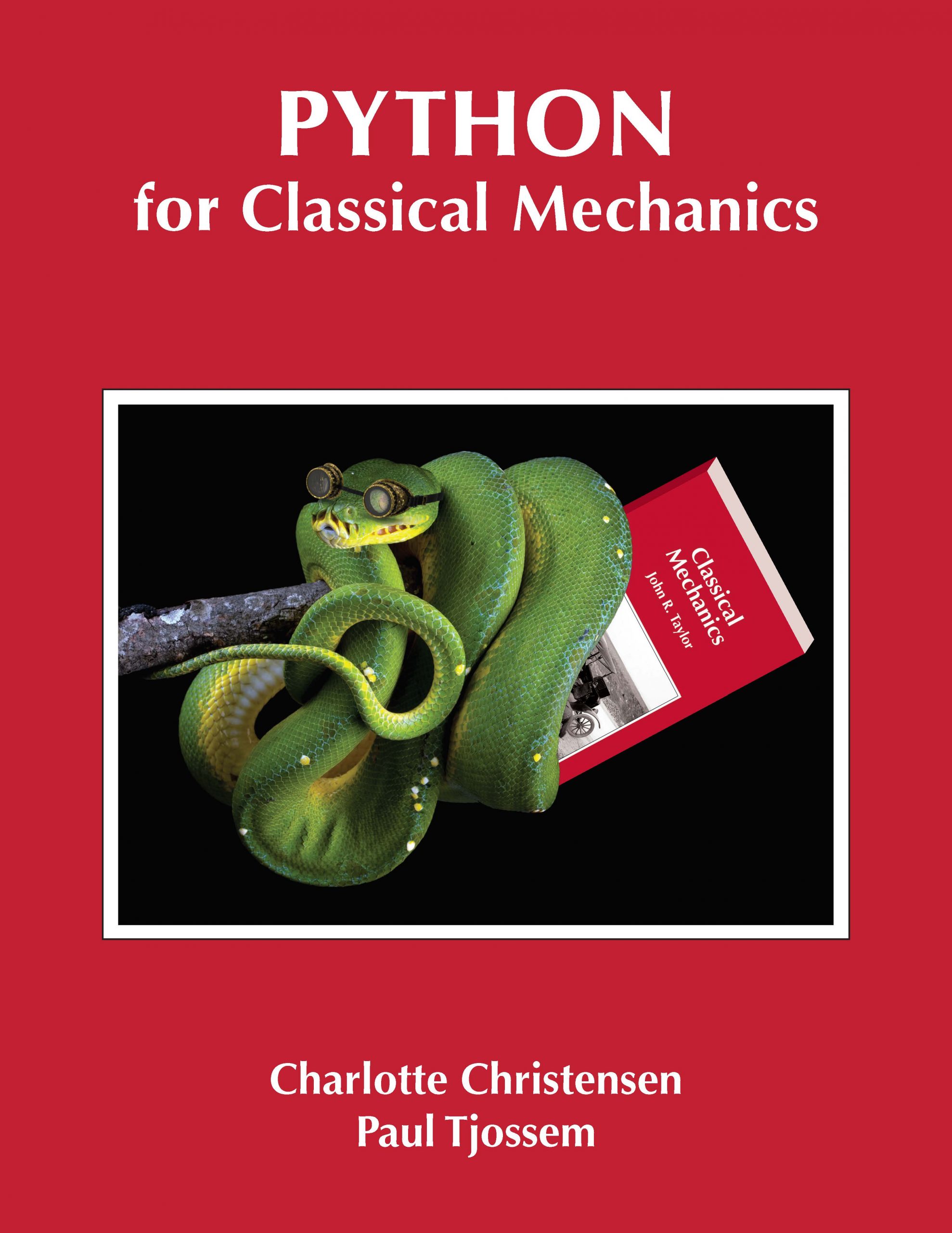
Python for Classical Mechanics
Newly Released
Designed to accompany John Taylor’s internationally best-selling Classical Mechanics, this text provides a series of interactive computational exercises in Python that analyze classical mechanical systems from both analytical and numerical perspectives. No pre-existing experience with Python is required, as this book integrates scientific programming instruction directly into the standard undergraduate classical mechanics physics course.
Summary
Contemporary physics relies heavily on computer programming for analyzing data and modeling systems, yet time constraints often prevent undergraduate physics students from taking the computer science courses needed to develop these skills. This textbook integrates scientific programming instruction directly into a standard undergraduate classical mechanics physics course. Built to accompany John Taylor’s popular Classical Mechanics, but compatible with other books, Python for Classical Mechanics provides a series of interactive Python computational exercises that analyze classical mechanical systems from both analytical and numerical perspectives. The exercises guide students chapter-by-chapter through modeling classical physics systems such as the simple pendulum at high angle, two or more gravitational bodies in orbit, and damped, driven oscillators leading to period-doubling and chaos.
Using guided instruction in critical programming techniques such as loops, logic, array manipulation, numerical integration, and data analysis and plotting to help intermediate physics, students gain proficiency in both analytical and computational methods. This book assumes no prior knowledge of programming on the part of the student and includes step-by-step instructions for starting the student programming in Python with the interactive Jupyter Notebook interface.
Table of Contents
Preface
Acknowledgements
1 Introduction
1.2 Who Is This Book For?
1.3 A Word of Encouragement to the Student
2 How To Use This Book
2.2 Scheduling
2.3 Working Through the Units
2.4 Relationship between Units
3 Description of Units
Introduction to Python
Taylor Series with Loops and Functions
Numerical Integration Applied to Projectile Motion
Projectile Motion with Drag
Launching a Rocket
Simple Pendulum with Large Angle Release
Comparing Data and Theory for Simple Pendulum
Oscillations in a Potential Well
Damped and Undamped Harmonic Oscillators
Driven Damped Harmonic Oscillator and Resonance
Brachistochrone Problem
Spherical Pendulum
Three-Body Problem
Orbits, Keplerian and Not
Motion on a Turntable
Coriolis Force on Earth
Principal Axes of a Cuboid
Precession of a Cuboid
Masses Connected with Springs
Damped Driven Pendulum
Bifurcation Diagram
State-Space Orbits and Poincaré Sections
Appendix 1: Using solve_ivp for Numerical Integration
Appendix 2: Basic Input/Output of Files in Python
Appendix 3: Creating Animations with FuncAnimation
4 Preparing to Use Jupyter Notebooks with Python
4.1 Installation on a Personal Computer/p>
4.1.2 Running Jupyter Notebook
4.1.3 Closing Jupyter Notebook
4.2 Using a Web Server to Run Jupyter Notebooks
4.2.2 Google Colab
5 Introduction to Python
5.1 Objectives
5.2 Working with Jupyter Notebook
5.2.2 The kernel
5.3 Introduction to Python Programming
5.3.2 Variables
5.3.3 Using Python for calculations
5.3.4 Order of operations, and left-right associativity
5.3.5 Data types
5.3.6 Formatting output
5.4 Lists and Arrays
5.4.2 Indexing and slicing
5.4.3 An aside on additional data types
5.5 Plotting
5.6 Check-out
6 Taylor Series with Loops and Functions
6.1 Objectives
6.2 Taylor Series
6.2.2 Taylor series for sin(x)
6.2.3 Taylor series about an arbitrary x value
6.3 New Programming Tools
6.3.2 Conditional statements
6.3.3 Loops
6.3.4 An aside on speed
6.3.5 Functions and other subroutines
6.4 Taylor Series using Loops, Functions, and Conditional Statements
6.5 Check-out
7 Numerical Integration Applied to Projectile Motion
7.1 Objectives
7.2 Simple Euler Integration of 2-D Projectile Motion
7.2.2 Accuracy of simple Euler integration
7.3 Improving the Simple Euler Integration Method: Euler Half-Step Integration
7.3.2 Applying improved Euler to projectile motion
7.4 Check-out
7.5 Challenge Problem
8 Projectile Motion with Drag
8.1 Objectives
8.2 Improved Euler Numerical Integration
8.3 Projectile Motion with Linear Drag
8.4 Quadratic Drag
8.4.2 Energy loss in one-dimensional motion
8.5 Linear and Quadratic Drag
8.6 Check-out
8.7 Challenge Problem
9 Launching a Rocket
9.1 Objectives
9.2 Motion of Rocket without Gravity
9.3 Introducing solve_ivp for a Rocket
9.3.2 Finding the solution with solve_ivp()
9.3.3 Accessing the solution from solve_ivp
9.3.4 Comparison between solve_ivp() and Improved Euler
9.4 Motion of a Rocket in a Constant Gravitational Field
9.4.2 Computational solution
9.5 Launching to the International Space Station
9.6 Check-out
9.7 Challenge Problem
10 Simple Pendulum with Large-Angle Release
10.1 Objectives
10.2 Simple Pendulum, Theory
10.2.2 Simple pendulum equation of motion
10.3 Numerical Solution for θ(t)
10.3.2 Finding the solution with solve_ivp()
10.4 Comparing Solutions for Simple Pendulum at Different Initial Angles
10.5 Period of Simple Pendulum as a Function of Release Angle
10.6 Check-out
10.7 Challenge Problems
11 Comparing Data and Theory for Simple Pendulum
11.1 Objectives
11.2 Computational Solution
11.3 Analytical Solution
11.4 Experimental Solution
11.4.2 Experimental data
11.5 Check-out
12 Oscillations in a Potential Well
12.1 Objectives
12.2 Potential Energy Function for an Oscillating Wheel
12.3 Analytical Approximation Using Taylor Series
12.3.2 Theoretical analysis of oscillations
12.4 Computational Solution for φ(t)
12.4.2 Computational solution for different mass ratios
12.4.3 Computational solution for different release angles
12.5 Check-out
12.6 Challenge Problems
13 Damped and Undamped Harmonic Oscillators
13.1 Objectives
13.2 Harmonic Motion without Damping
13.2.2 Numerical solution
13.3 Damped Harmonic Oscillator
13.3.2 Case 2: Large damping, β2 > ω20
13.3.3 Case 3: Critical damping, β2 = ω20
13.3.4 Case 4: Underdamping, β2 < ω20
13.4 Check-out
13.5 Challenge Problems
14 Driven Damped Harmonic Oscillator and Resonance
14.1 Objectives
14.2 Motion of a Driven Damped Harmonic Oscillator
14.3 Amplitude of Driven Damped Oscillations at Resonance
14.4 Phase of Driven Damped Oscillations
14.5 The Phase Dependence
14.6 Amplitude as a Function of Driver Frequency
14.7 Creating a Numerical Resonance Curve by Plotting the Maximum Amplitude vs. Frequency
14.7.2 Now for the geometric interpretation
14.8 Check-out
14.9 Challenge Problems
14.9.2 Challenge Problem 2, Effect of β on the resonance curve
14.9.3 Challenge Problem 3, Multiprocessing for multiple resonance curves
14.10 Contents of resonance_for_multi_processing_solvers.py
15 Brachistrochrone Problem
15.1 Objectives
15.2 Introducing the Cycloid
15.3 Cycloidal Path Length
15.4 Travel Time
15.4.2 Time taken for an arbitrary starting angle
15.4.3 Numerical solution
15.5 An Animation
15.6 Check-out
15.7 Challenge Problem
16 Spherical Pendulum
16.2 Equations of Motion for a Spherical Pendulum
16.3 Validating Your Code with Special Cases
16.4 Varying Initial Velocity
16.5 Conservation of Generalized Momentum
16.6 Near-Conical Motion
16.7 Check-out
16.8 Challenge Problem
17 The Three-Body Problem
17.1 Objectives
17.2 Solving the Two-Body Problem Numerically for a Circular Orbit
17.3 Numerical Integration of the Three-Body Problem
17.3.2 Mystery system
17.3.3 Plotting in the center-of-mass frame of reference
17.4 Making a Movie
17.5 Three Dimensions
17.6 Check-out
17.7 Challenge Problem
18 Orbits, Keplerian and Not
18.1 Objectives
18.2 Circular Keplerian Orbit (ϵ = 0)
18.3 Numerical Solution
18.4 An Elliptical Orbit
18.5 Hyperbolic Orbits
18.6 Comparing with Pluto Ephemeris
18.7 Non-Keplerian Orbits
18.8 Check-out
18.9 Challenge Problems
19 Motion on a Turntable
19.1 Objectives
19.2 Preliminary Questions
19.3 Framing the Problem
19.3.2 Setting the initial conditions and other physical parameters
19.3.3 Numerically solving the equations of motion
19.3.4 Comparing the trajectory in the rotating reference frame to that in a fixed inertial reference frame
19.3.5 Explore different initial conditions
19.4 Animating the Trajectory
19.5 Check-out
19.6 Challenge Problems
20 Coriolis Force on Earth
20.1 Objectives
20.2 Equations of Motion
20.3 Solving the Equations of Motion
20.3.2 Solving the equations of motion for a set of initial conditions
20.3.3 Plotting on the surface of a sphere
20.4 Verifying Your Code
20.5 Explore Different Initial Conditions
20.6 Integrate with Realistic Parameters
20.7 Check-out
20.8 Challenge Problems
21 Principal Axes of a Cuboid
21.1 Objectives
21.2 Coding Techniques Preamble
21.2.2 Classes
21.3 Moment of Inertia Tensor and Angular Momentum
21.3.2 Creating a class
21.4 Finding the Principal Axes
21.5 Check-out
21.6 Challenge Problem
22 Precession of a Cuboid
22.1 Objectives
22.2 Creating and Importing Modules
22.3 Euler’s Equations
22.4 Check-out
22.5 Template Code for principal_axes.py
23 Masses Connected with Springs
23.1 Objectives
23.2 Two Carts Connected and Attached between Two Walls by Three Springs
23.3 Identical Masses and Springs
23.3.2 Numerical solution
23.3.3 Solving the eigenvalue problem numerically
23.4 Weak Coupling, an Illustration of Beats
23.5 Fourier Analysis
23.6 Check-out
23.7 Challenge Problems
24 Damped Driven Pendulum
24.1 Objectives
24.2 Equation of Motion
24.3 Numerical Solution
24.3.2 Numerically solving the equation of motion
24.3.3 Coding style
24.4 Behavior with Increasing Values of Driving
24.4.2 Intermediate and strong driving
24.5 Sensitivity to Initial Conditions
24.6 Check-out
24.7 Challenge Problem
25 Bifurcation Diagram
25.2 Setup
25.3 One-Point Bifurcation Diagram
25.4 Creating the Full Bifurcation Diagram
25.5 Features of the Bifurcation Diagram
25.6 Class Parallel Programming Project
25.7 Check-out
25.8 Challenge Problem
25.9 Template Code for damped_driven_pendulum.py
26 State-Space Orbits and Poincaré Sections
26.2 Setup
26.3 State-Space
26.4 Poincaré Sections
26.5 Strange Attractors
26.6 Check-out
27 Appendix 1: Using solve_ivp for Numerical Integration
27.1 Using solve_ivp()
27.1.2 Accuracy
27.1.3 Checking for events
28 Appendix 2: Basic Input/Output of Files in Python
28.1 Read/Write to a File Handle
28.1.2 Read
28.2 Using NumPy for Reading and Writing Data Arrays
28.3 Pandas
28.4 Binary Data
28.4.2 Reading binary data
29 Appendix 3: Creating Animations with FuncAnimation
29.1 Overview
29.2 Walk-through Example
29.2.2 Frame functions
29.3 Call the Animator
Index


